Reimplementation + Explorations
Original link: https://inst.eecs.berkeley.edu/~cs180/fa23/upload/files/proj6/yifengwang/#part-2
1. Introduction
A Neural Algorithm of Artistic Style, by Gatys et al., was a seminal work in the field of neural style transfer. On a very high level, the approach they introduced was to use CNNs to separate and recombine content and style. I am especially impressed by the novel approach and the aesthetic pleasure from the synthesized images. In this part of the final project, I reimplemented their approach while introducing some personal experimentation.
Here are links to the original paper and two PyTorch tutorials (PyTorch and d2l) that were helpful in guiding my implementation.
In order to use GPU compute, I set up my environment on Azure ML Notebook, utilizing some free credits I had from previous work (thanks Microsoft!). I also set up a project in Weights & Biases to log my results in each run. It turned out logging hyperparameters and synthesized images was extremely important - when I was stuck at some uninteresting results, looking at experiment data helped me figure out the correct parameters to choose.
Reading the paper, I thought the most interesting part comes from realizing we are not training the neural network itself in the traditional sense. What is being optimized instead is the synthesized image. As discussed by the authors, there usually exists no such image that perfectly captures the content of one image and the style of the other. But as we minimize the loss function, the synthetic image we generated becomes more perceptually appealing.
2. The VGG Network
We use a pre-trained convolutional neural network called VGG-19. The network is originally used for object recognition, outperforming many previous results on ImageNet at the time of its release. This made the network suitable for our task - with its object recognition abilities, it can “capture the high-level content in terms of objects and their arrangement in the input image but do not constrain the exact pixel values of the reconstruction.” We initialize the network with pre-trained weights from VGG19_Weights.IMAGENET1K_V1.
We use the VGG network to extract features from the content image and the style image. Using these “feature maps” we can calculate content and style loss.
3. Loss Functions
The content generation problem is easy - we define content loss using the MSE loss between the synthesized image’s features and the original content image’s features. Style features, on the other hand, are difficult. For each layer used in style representation, we need to compute the Gram matrix. The elements of the Gram matrix represent the correlations between the activations of different filters in the layer. These correlations capture the texture and visual patterns that are characteristic of the style of the image.
In addition to content and style loss described in the original paper, total variation loss (tv_loss) was also computed. This is meant to minimize the amount of high frequency artifacts in the synthetic image.
4. Training
In earlier training runs, I failed to get satisfying results even after 1,500 epochs. By examining my hyperparameters and the way the images changed, I noticed the content features were reconstructed well, but the stylistic elements were not showing. I assigned a heavier weight to style (1e6 instead of 1e3 or 1e4) and the model started generating interesting results.
5. Results
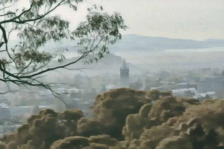
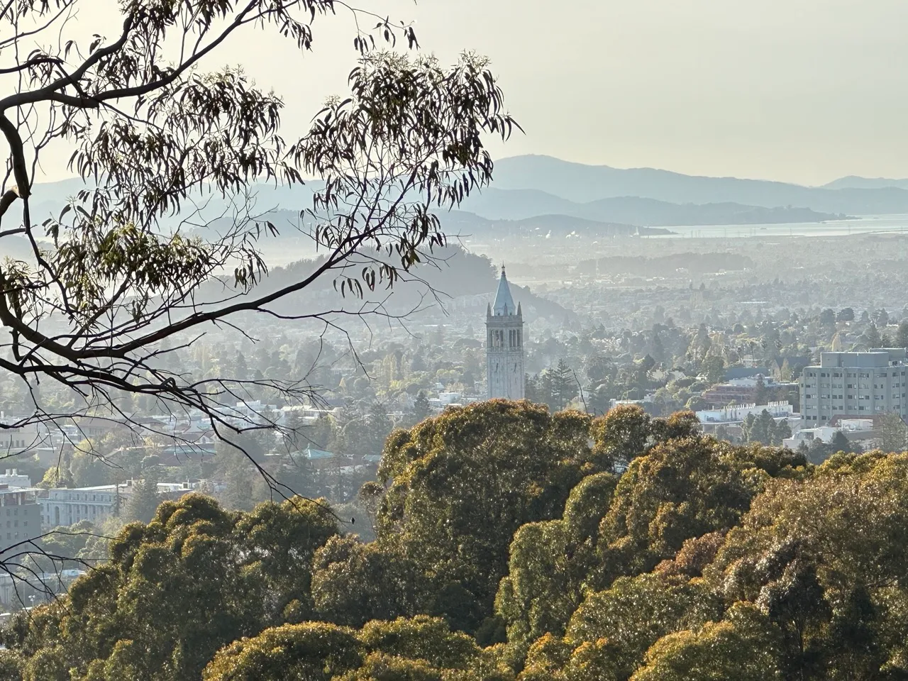
Content Images
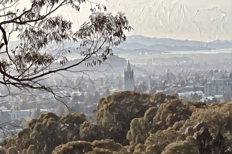
Berkeley, CA
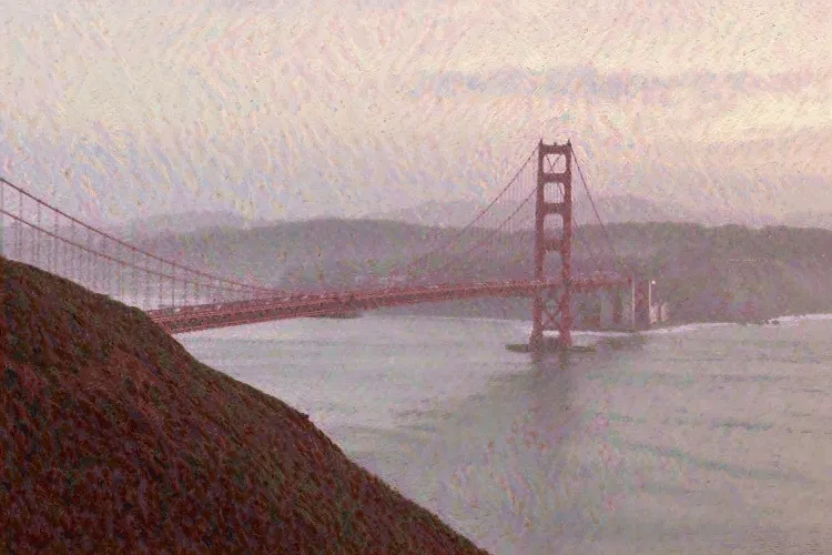
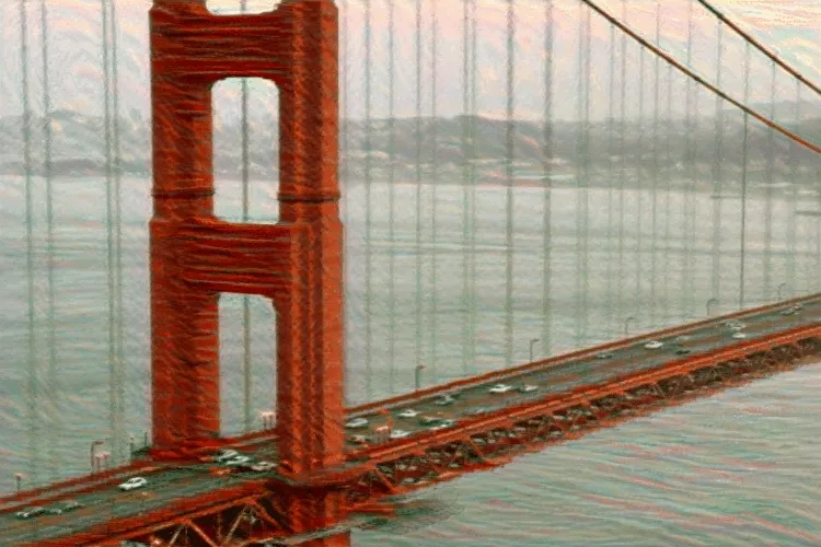
Golden Gate Bridge 1
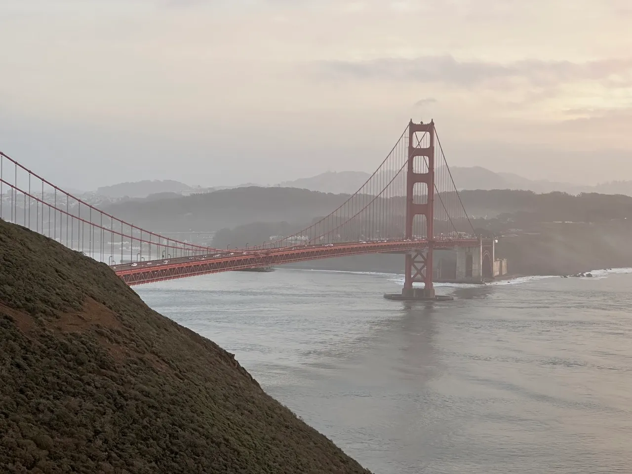
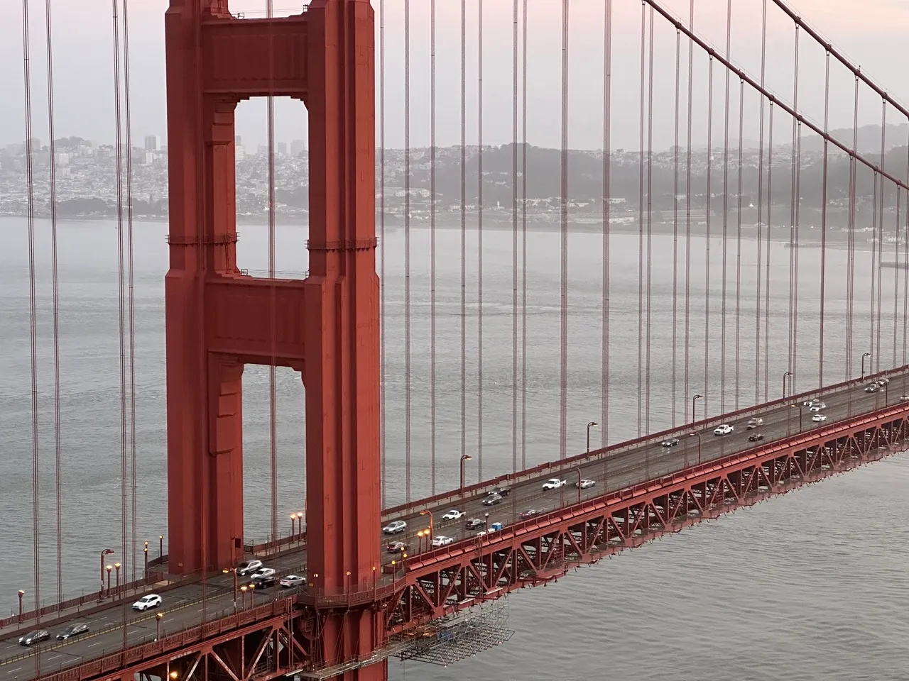
Golden Gate Bridge 2
Style Images
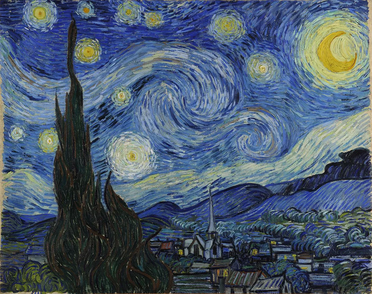
The Starry Night, Vincent van Gogh
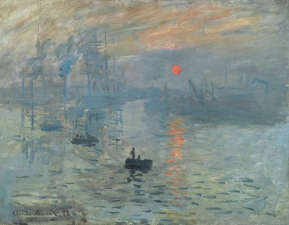
Impression, Sunrise, Claude Monet
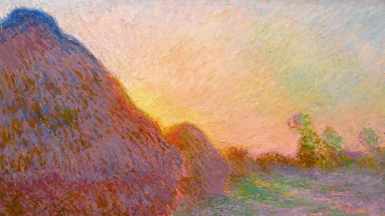
Haystacks, Claude Monet
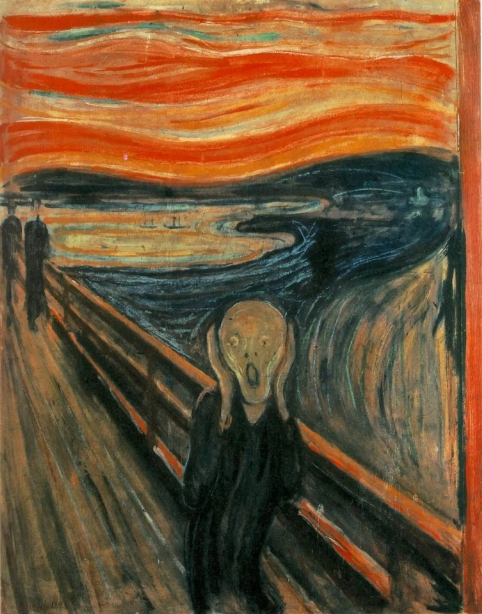
The Scream, Edvard Munch
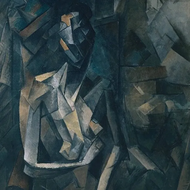
Figure, Pablo Picasso
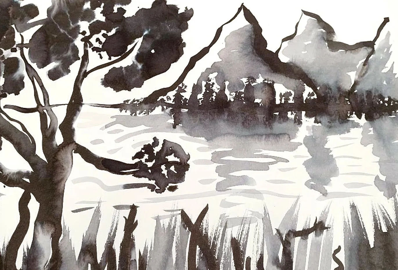
Journey to the East, Bukang Y. Kim
Input (Synthetic) Images
All of these are GIFs showing the gradual synthesis of the combined image. You might have to stare at them a little to spot the change!
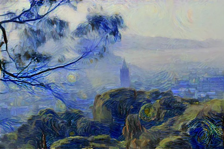
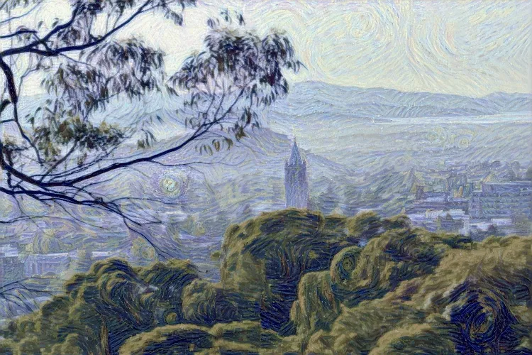
Berkeley + Starry
Berkeley + Scream
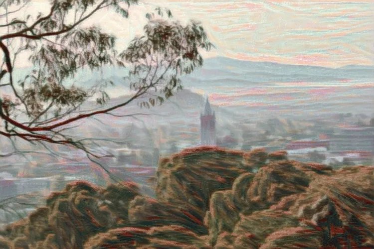
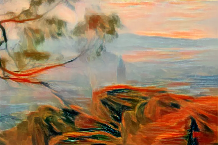
Berkeley + Sunrise
Berkeley + Cubism
Bridge + Scream
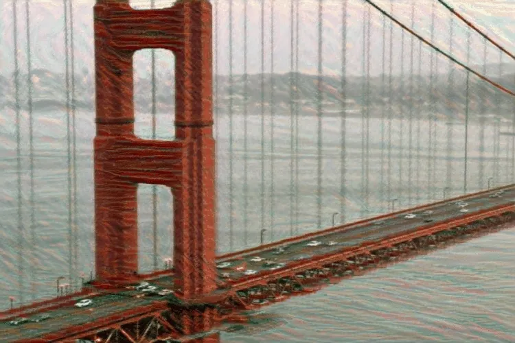
Bridge 2 + Haystacks
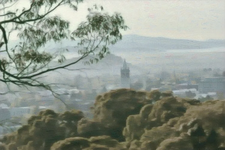
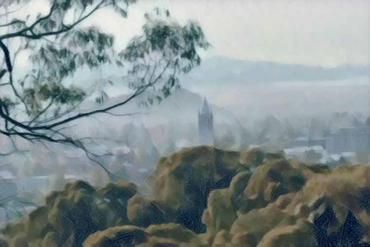
Berkeley + Ink Wash
My comment on the last synthetic image, which combines Berkeley and Ink Wash styles, is that the model captures the style only very superficially. It does not abstract away details adequately as is common in most ink wash paintings. But of course, this level of reasoning or artistic interpretation isn’t what we’d expect from this current model.
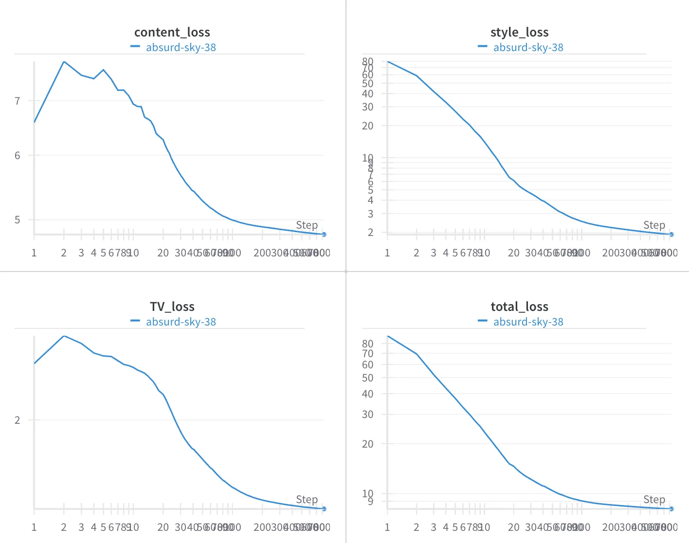
I also recorded hyperparameters and losses for each run. Here are the results for the Bridge + Scream example shown above.
Shuffling Layers
I also compared the results from different selections of layers from the VGG network.
Approach 1
style_layers = [0, 5, 10, 19, 28]
content_layers = [25]
Approach 2
style_layers = [2, 7, 12, 21, 30]\
content_layers = [22, 25]
I like the result from approach 2 better because
- content features seem more detailed, and
- it is more artistically expressive.
For this following example, there isn’t a huge difference between the two approaches except for the colors.
Approach 1
style_layers = [0, 5, 10, 19, 28]
content_layers = [25]
Approach 2
style_layers = [2, 7, 12, 21, 30]
content_layers = [22, 25]